
It’s commonly assumed that prices have a Gaussian, or normal, Probability Density Function (PDF). A Gaussian PDF is the familiar bell-shaped curve where 68% of all samples fall within one standard deviation about the mean. This is a really bad assumption and the reason many trading indicators fail to produce as expected.
Suppose prices behave as a square wave. If you tried to use the price crossing a moving average as a trading system you would be destined for failure because the price has already switched to the opposite value by the time the movement is detected. There are only two price values. Therefore, the probability distribution is 50% that the price will be at one value or the other. There are no other possibilities. The probability distribution of the square wave is shown in Figure 1. Clearly, this probability function is a long way from Gaussian.

Figure 1. The probability distribution of a square wave only has two values.
There is no great mystery about the meaning of a probability density or how it is computed. It is simply the likelihood the price will assume a given value. Think of it this way: Construct any waveform you choose by arranging beads strung on a series of parallel horizontal wires. After the waveform is created, turn the frame so the wires are vertical. All the beads will fall to the bottom, and the number of beads on each wire will stack up to demonstrate the probability of the value represented by each wire.
I used a slightly more sophisticated computer code, but nonetheless the same idea, to create the probability distribution of a sine wave in Figure 2. In this case, I used a total of 2000 “beads.” This PDF may be surprising, but if you stop and think about it, you will realize that most of the sampled data points of a sine wave occur near the maximum and minimum extremes. The PDF of a simple sine wave cycle is not at all similar to a Gaussian PDF. In fact, cycle PDFs are more closely related to those of a square wave. The high probability of a cycle being near the extreme values is one of the reasons why cycles are difficult to trade. About the only way to successfully trade a cycle is to take advantage of the short-term coherency and predict the cyclic turning point.
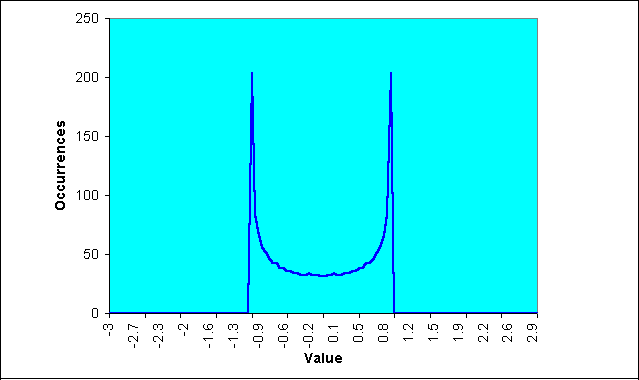
Figure 2. A sinewave cycle probability density function does not resemble a gaussian probability density function.
The Fisher Transform changes the PDF of any waveform so that the transformed output has an approximately Gaussian PDF. The Fisher Transform equation is:
![]()
Where:
x is the input
y is the output
ln is the natural logarithm
The transfer function of the Fisher Transform is shown in Figure 3.
Figure 3. The nonlinear transfer of the fisher transform converts inputs [x-axis] to outputs [y-axis] having a nearly gaussian probability distribution function.
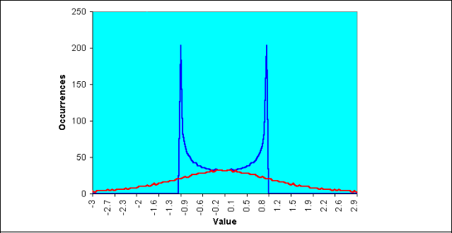
The fisher transformed sinewave has a nearly gaussian probability density function shape.
So what does this mean in trading? If the prices are normalized to fall within the range from –1 to +1 and subjected to the Fisher Transform, the extreme price movements are relatively rare events. This means the turning points can be clearly and unambiguously identified. The EasyLanguage code to do this is shown in Code Listing 1. The Stochastic indicator is computed to swing between the –1 and +1 limits. The Stochastic is smoothed with an EMA and amplified to mitigate smoothing losses. The Fisher Transform is computed to be the variable “Fisher”.
//Stochastic and Fisher Transform
//(c) 2016 John F. Ehlers
Inputs:
Length(9);
Vars:
count(0),
HH(0),
LL(0),
Stoc(0),
SlowStoc(0),
Fisher(0);
HH = High;
LL = Low;
For count = 0 to Length – 1 Begin
If High[count] > HH Then HH = High[count];
If Low[count] < LL Then LL = Low[count];
End;
Stoc = 2*(Close – LL) / (HH-LL) – 1;
//Smooth with EMA and scale for filter loss
SlowStoc = .2*1.5*Stoc + .8*SlowStoc;
//Apply Fisher Transform
If SlowStoc > .999 Then SlowStoc = .999;
If SlowStoc < -.999 Then SlowStoc = -.999;
Fisher = Log( (1 + SlowStoc) / (1 – SlowStoc) ) * .5;
Plot1(Fisher);
Plot2(0);
Plot6(2);
Code Listing 1. EasyLanguage code for a stochastic indicator and its fisher transform.
The 9 day Stochastic is plotted in the first subgraph below the price bars in Figure 5. Note that the turning points are not sharp and distinct. The Fisher Transform of the 9 day Stochastic is plotted in the second subgraph below the price bars.
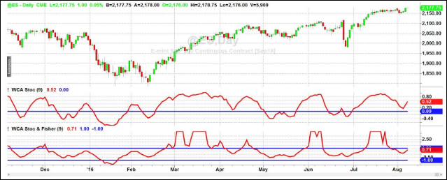
Figure 5. The fisher transform clearly identifies reversion to the mean.
It is better to wait for confirmation when making a trade. Confirmation for entering a long position occurs when the waveform crosses over the lower threshold and crosses under the upper threshold for entering a short position. A short trade is signaled in December 2015. A long trade (and short exit) is signaled in January 2016. The exit (and reversal to a short position) is signaled twice in April 2016. Additional short entries are signaled in June 2016 and in late July 2016. As shown by the June and July signals, the Fisher Transform should not be used alone. Rather, it is another arrow in your quiver of techniques.
CONCLUSIONS
Prices do not have a Gaussian PDF. By normalizing prices or creating a normalized indicator such as the RSI or Stochastic, and applying the Fisher Transform, a nearly Gaussian PDF can be created. Such a transformed output creates the peak swings as relatively rare events. The sharp turning points of these peak swings clearly and unambiguously identify price reversals in a timely manner. As a result, superior discretionary trading can be expected and higher performing mechanical trading systems can be developed by using the Fisher Transform.
For a closer look at the Fisher Transform and using the Inverse Fisher Transform, click here.